Aggregation Browsing and Aggregations

The main purpose of the Cubes framework is aggregation and browsing through the aggregates. In this chapter we are going to demonstrate how basic aggregation is done.

Note

See the backend documentation for reference.

ROLAP with SQL backend

Following examples will show:

• how to build a model programmatically
• how to create a model with flat dimensions
• how to aggregate whole cube
• how to drill-down and aggregate through a dimension

The example data used are IBRD Balance Sheet taken from The World Bank. Backend used for the examples is sql.browser.

Create a tutorial directory and download this example file.

Start with imports:

>>> from sqlalchemy import create_engine
>>> from cubes.tutorial.sql import create_table_from_csv

Note

Cubes comes with tutorial helper methods in cubes.tutorial. It is advised not to use them in production, they are provided just to simplify learner’s life.

Prepare the data using the tutorial helpers. This will create a table and populate it with contents of the CSV file:

>>> engine = create_engine('sqlite:///data.sqlite')
... create_table_from_csv(engine,
...                       "data.csv",
...                       table_name="irbd_balance",
...                       fields=[
...                             ("category", "string"),
...                             ("category_label", "string"),
...                             ("subcategory", "string"),
...                             ("subcategory_label", "string"),
...                             ("line_item", "string"),
...                             ("year", "integer"),
...                             ("amount", "integer")],
...                       create_id=True
...                   )

Download the example model and save it. Load the model:

>>> import cubes
>>> model = cubes.load_model("model.json")

Check whether the model is valid with model.is_valid() - should return True.

>>> model.is_valid()
True

Create a workspace and get a browser instance (in this example it is SQL backend):

>>> workspace = cubes.create_workspace("sql.star", model, engine=engine)

Get a cube and browser for the cube:

>>> cube = model.cube("irbd_balance")
>>> browser = workspace.browser(cube)

cell defines context of interest - part of the cube we are looking at. We start with whole cube:

>>> cell = cubes.Cell(cube)

Compute the aggregate. Measure fields of aggregation result have aggregation suffix. Also a total record count within the cell is included as record_count.

>>> result = browser.aggregate(cell)
>>> result.summary["record_count"]
62
>>> result.summary["amount_sum"]
1116860

Now try some drill-down by year dimension:

>>> result = browser.aggregate(cell, drilldown=["year"])
>>> for record in result.drilldown:
...     print record
{u'record_count': 31, u'amount_sum': 550840, u'year': 2009}
{u'record_count': 31, u'amount_sum': 566020, u'year': 2010}

Drill-dow by item category:

>>> result = browser.aggregate(cell, drilldown=["item"])
>>> for record in result.drilldown:
...     print record
{u'item.category': u'a', u'item.category_label': u'Assets', u'record_count': 32, u'amount_sum': 558430}
{u'item.category': u'e', u'item.category_label': u'Equity', u'record_count': 8, u'amount_sum': 77592}
{u'item.category': u'l', u'item.category_label': u'Liabilities', u'record_count': 22, u'amount_sum': 480838}

Aggregations and Aggregation Result

Aggregate types depend on the backend, however there is at least one that should be supported by all backends: sum. The SQL StarBrowser supports also min, max and avg. In some databases, such as PostgreSQL, stddev and variance can be used.

Relevant aggregations for a measure can be specified in the model description:

"measures": [
    {
        "name": "amount",
        "aggregations": ["sum", "min", "max"]
    }
]

The resulting aggregated attribute name will be constructed from the measure name and aggregation suffix, for example the mentioned amount will have three aggregates in the result: amount_sum, amount_min and amount_max in the case described above.

Result of aggregation is a structure containing: summary - summary for the aggregated cell, drilldown - drill down cells, if was desired, and total_cell_count - total cells in the drill down, regardless of pagination.

Cell Details

When we are browsing a cube, the cell provides current browsing context. For aggregations and selections to happen, only keys and some other internal attributes are necessary. Those can not be presented to the user though. For example we have geography path (country, region) as ['sk', 'ba'], however we want to display to the user Slovakia for the country and Bratislava for the region. We need to fetch those values from the data store. Cell details is basically a human readable description of the current cell.

For applications where it is possible to store state between aggregation calls, we can use values from previous aggregations or value listings. Problem is with web applications - sometimes it is not desirable or possible to store whole browsing context with all details. This is exact the situation where fetching cell details explicitly might come handy.

Note

The Original browser added cut information in the summary, which was ok when only point cuts were used. In other situations the result was undefined and mostly erroneous.

The cell details are now provided separately by method cubes.AggregationBrowser.cell_details() which has Slicer HTTP equivalent /cell or {"query":"detail", ...} in /report request (see the server documentation for more information).

For point cuts, the detail is a list of dictionaries for each level. For example our previously mentioned path ['sk', 'ba'] would have details described as:

[
    {
        "geography.country_code": "sk",
        "geography.country_name": "Slovakia",
        "geography.something_more": "..."
        "_key": "sk",
        "_label": "Slovakia"
    },
    {
        "geography.region_code": "ba",
        "geography.region_name": "Bratislava",
        "geography.something_even_more": "...",
        "_key": "ba",
        "_label": "Bratislava"
    }
]

You might have noticed the two redundant keys: _key and _label - those contain values of a level key attribute and level label attribute respectively. It is there to simplify the use of the details in presentation layer, such as templates. Take for example doing only one-dimensional browsing and compare presentation of “breadcrumbs”:

labels = [detail["_label"] for detail in cut_details]

Which is equivalent to:

levels = dimension.hierarchy().levels()
labels = []
for i, detail in enumerate(cut_details):
    labels.append(detail[level[i].label_attribute.ref()])

Note that this might change a bit: either full detail will be returned or just key and label, depending on an option argument (not yet decided).

Hierarchies, levels and drilling-down

• how to create a hierarchical dimension
• how to do drill-down through a hierarchy
• detailed level description

We are going to use very similar data as in the previous examples. Difference is in two added columns: category code and sub-category code. They are simple letter codes for the categories and subcategories. Download this example file.

Hierarchy

Some dimensions can have multiple levels forming a hierarchy. For example dates have year, month, day; geography has country, region, city; product might have category, subcategory and the product.

In our example we have the item dimension with three levels of hierarchy: category, subcategory and line item:

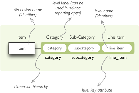
Item dimension hierarchy.

The levels are defined in the model:

"levels": [
    {
        "name":"category",
        "label":"Category",
        "attributes": ["category"]
    },
    {
        "name":"subcategory",
        "label":"Sub-category",
        "attributes": ["subcategory"]
    },
    {
        "name":"line_item",
        "label":"Line Item",
        "attributes": ["line_item"]
    }
]

You can see a slight difference between this model description and the previous one: we didn’t just specify level names and didn’t let cubes to fill-in the defaults. Here we used explicit description of each level. name is level identifier, label is human-readable label of the level that can be used in end-user applications and attributes is list of attributes that belong to the level. The first attribute, if not specified otherwise, is the key attribute of the level.

Other level description attributes are key and label_attribute`. The key specifies attribute name which contains key for the level. Key is an id number, code or anything that uniquely identifies the dimension level. label_attribute is name of an attribute that contains human-readable value that can be displayed in user-interface elements such as tables or charts.

Preparation

Again, in short we need:

• data in a database
• logical model (see model file) prepared with appropriate mappings
• denormalized view for aggregated browsing (optional)

Drill-down

Drill-down is an action that will provide more details about data. Drilling down through a dimension hierarchy will expand next level of the dimension. It can be compared to browsing through your directory structure.

We create a function that will recursively traverse a dimension hierarchy and will print-out aggregations (count of records in this example) at the actual browsed location.

Attributes

• cell - cube cell to drill-down
• dimension - dimension to be traversed through all levels
• path - current path of the dimension

Path is list of dimension points (keys) at each level. It is like file-system path.

def drill_down(cell, dimension, path=[]):

Get dimension’s default hierarchy. Cubes supports multiple hierarchies, for example for date you might have year-month-day or year-quarter-month-day. Most dimensions will have one hierarchy, thought.

hierarchy = dimension.hierarchy()

Base path is path to the most detailed element, to the leaf of a tree, to the fact. Can we go deeper in the hierarchy?

if hierarchy.path_is_base(path):
    return

Get the next level in the hierarchy. levels_for_path returns list of levels according to provided path. When drilldown is set to True then one more level is returned.

levels = hierarchy.levels_for_path(path,drilldown=True)
current_level = levels[-1]

We need to know name of the level key attribute which contains a path component. If the model does not explicitly specify key attribute for the level, then first attribute will be used:

level_key = dimension.attribute_reference(current_level.key)

For prettier display, we get name of attribute which contains label to be displayed for the current level. If there is no label attribute, then key attribute is used.

level_label = dimension.attribute_reference(current_level.label_attribute)

We do the aggregation of the cell...

Note

Shell analogy: Think of ls $CELL command in commandline, where $CELL is a directory name. In this function we can think of $CELL to be same as current working directory (pwd)

result = browser.aggregate(cell, drilldown=[dimension])

for record in result.drilldown:
    print "%s%s: %d" % (indent, record[level_label], record["record_count"])
    ...

And now the drill-down magic. First, construct new path by key attribute value appended to the current path:

drill_path = path[:] + [record[level_key]]

Then get a new cell slice for current path:

drill_down_cell = cell.slice(dimension, drill_path)

And do recursive drill-down:

drill_down(drill_down_cell, dimension, drill_path)

The whole recursive drill down function looks like this:

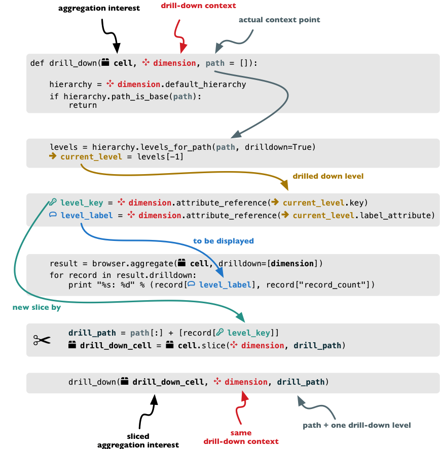
Recursive drill-down explained

Whole working example can be found in the tutorial sources.

Get the full cube (or any part of the cube you like):

cell = browser.full_cube()

And do the drill-down through the item dimension:

drill_down(cell, cube.dimension("item"))

The output should look like this:

a: 32
    da: 8
        Borrowings: 2
        Client operations: 2
        Investments: 2
        Other: 2
    dfb: 4
        Currencies subject to restriction: 2
        Unrestricted currencies: 2
    i: 2
        Trading: 2
    lo: 2
        Net loans outstanding: 2
    nn: 2
        Nonnegotiable, nonintrest-bearing demand obligations on account of subscribed capital: 2
    oa: 6
        Assets under retirement benefit plans: 2
        Miscellaneous: 2
        Premises and equipment (net): 2

Note that because we have changed our source data, we see level codes instead of level names. We will fix that later. Now focus on the drill-down.

See that nice hierarchy tree?

Now if you slice the cell through year 2010 and do the exact same drill-down:

cell = cell.slice("year", [2010])
drill_down(cell, cube.dimension("item"))

you will get similar tree, but only for year 2010 (obviously).

Level Labels and Details

Codes and ids are good for machines and programmers, they are short, might follow some scheme, easy to handle in scripts. Report users have no much use of them, as they look cryptic and have no meaning for the first sight.

Our source data contains two columns for category and for subcategory: column with code and column with label for user interfaces. Both columns belong to the same dimension and to the same level. The key column is used by the analytical system to refer to the dimension point and the label is just decoration.

Levels can have any number of detail attributes. The detail attributes have no analytical meaning and are just ignored during aggregations. If you want to do analysis based on an attribute, make it a separate dimension instead.

So now we fix our model by specifying detail attributes for the levels:

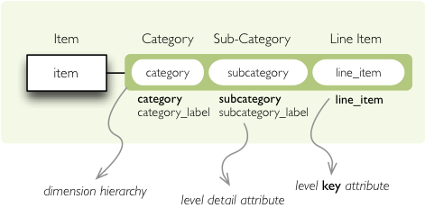
Attribute details.

The model description is:

"levels": [
        {
            "name":"category",
            "label":"Category",
            "label_attribute": "category_label",
            "attributes": ["category", "category_label"]
        },
        {
            "name":"subcategory",
            "label":"Sub-category",
            "label_attribute": "subcategory_label",
            "attributes": ["subcategory", "subcategory_label"]
        },
        {
            "name":"line_item",
            "label":"Line Item",
            "attributes": ["line_item"]
        }
    ]
}

Note the label_attribute keys. They specify which attribute contains label to be displayed. Key attribute is by-default the first attribute in the list. If one wants to use some other attribute it can be specified in key_attribute.

Because we added two new attributes, we have to add mappings for them:

"mappings": { "item.line_item": "line_item",
              "item.subcategory": "subcategory",
              "item.subcategory_label": "subcategory_label",
              "item.category": "category",
              "item.category_label": "category_label"
             }

Now the result will be with labels instead of codes:

Assets: 32
    Derivative Assets: 8
        Borrowings: 2
        Client operations: 2
        Investments: 2
        Other: 2
    Due from Banks: 4
        Currencies subject to restriction: 2
        Unrestricted currencies: 2
    Investments: 2
        Trading: 2
    Loans Outstanding: 2
        Net loans outstanding: 2
    Nonnegotiable: 2
        Nonnegotiable, nonintrest-bearing demand obligations on account of subscribed capital: 2
    Other Assets: 6
        Assets under retirement benefit plans: 2
        Miscellaneous: 2
        Premises and equipment (net): 2

Implicit hierarchy

Try to remove the last level line_item from the model file and see what happens. Code still works, but displays only two levels. What does that mean? If metadata - logical model - is used properly in an application, then application can handle most of the model changes without any application modifications. That is, if you add new level or remove a level, there is no need to change your reporting application.

Summary

• hierarchies can have multiple levels
• a hierarchy level is identifier by a key attribute
• a hierarchy level can have multiple detail attributes and there is one special detail attribute: label attribute used for display in user interfaces

Multiple Hierarchies

Dimension can have multiple hierarchies defined. To use specific hierarchy for drilling down:

result = browser.aggregate(cell, drilldown = [("date", "dmy", None)])

The drilldown argument takes list of three element tuples in form: (dimension, hierarchy, level). The hierarchy and level are optional. If level is None, as in our example, then next level is used. If hierarchy is None then default hierarchy is used.

To sepcify hierarchy in cell cuts just pass hierarchy argument during cut construction. For example to specify cut through week 15 in year 2010:

cut = cubes.PointCut("date", [2010, 15], hierarchy="ywd")

Note

If drilling down a hierarchy and asking cubes for next implicit level the cuts should be using same hierarchy as drilldown. Otherwise exception is raised. For example: if cutting through year-month-day and asking for next level after year in year-week-day hierarchy, exception is raised.